Code
library(Rcpp)
source("./source/data_generation.r")
source("./source/greedy_cp_selection.r")
Rcpp::sourceCpp("./source/greedy_cp_selection.cpp")library(Rcpp)
source("./source/data_generation.r")
source("./source/greedy_cp_selection.r")
Rcpp::sourceCpp("./source/greedy_cp_selection.cpp")This notebook demonstrates a Bayesian changepoint detection algorithm for histogram-valued time series. It is based on a greedy search tailored for transactional price data with varying pricing regimes.
We model the price distribution of a product as a histogram over discrete price points, because in B2C scenarios, only a few specifc prices are available at any given time. Some customer groups may be offered a discount, while most purchase at the list price. Modeling daily means or medians may lose the multimodal structure that matters most for detecting pricing regimes. Histogram-valued preserve the full distributional shape, making it possible to detect subtle regime shifts such as list price changes or availability of discounts. The method is useful for detecting changes in pricing regimes, such as list price changes, promotions, or changes in the availability of discounts.
Each day is represented by a histogram over discrete price points. The time series is transformed into a histogram-valued sequence, represented as a matrix of counts. We assume that pricing follows distinct pricing regimes, each associated with a different price distribution. Changes in pricing regime occur when the pricing of a product undergoes a meaningful change — such as list price changes, promotions, or changes in the availability of discounts. Changepoints are defined as time indices where the underlying price distribution regime changes, leading to a change in relative frequency of price points.
The synthetic data used in this notebook simulates 800 days of pricing activity, segmented into 10 regimes characterized by different list prices, discounts, and discount availability
set.seed(123)

segments <- data.frame(
             start_day = c(1,  90, 250, 300, 400, 500, 550, 600, 700, 750),
            list_price = c(5,    6,   6,   6,   6, 5.5, 5.5, 5.5, 7, 7),
        discount_price = c(4,    4,   5,   5,   5, 4.5, 4.5, 4.5, 2, 2),
   discount_percentage = c(.25, .1,  .1, .25,  .5, .01, .03, .15,.3, .4)
)

n_days <- 800
lambda_qty <- 20
df <- generate_transaction_prices(segments, n_days, lambda_qty, seed = 123)
hist <- compute_price_histogram(df)
actual_changepoints <- segments$start_day[-1]-0.5

knitr::kable(segments, caption = "Price Regimes Overview")| start_day | list_price | discount_price | discount_percentage |
|---|---|---|---|
| 1 | 5.0 | 4.0 | 0.25 |
| 90 | 6.0 | 4.0 | 0.10 |
| 250 | 6.0 | 5.0 | 0.10 |
| 300 | 6.0 | 5.0 | 0.25 |
| 400 | 6.0 | 5.0 | 0.50 |
| 500 | 5.5 | 4.5 | 0.01 |
| 550 | 5.5 | 4.5 | 0.03 |
| 600 | 5.5 | 4.5 | 0.15 |
| 700 | 7.0 | 2.0 | 0.30 |
| 750 | 7.0 | 2.0 | 0.40 |
The plot below shows the synthetic data set, with the actual changepoints marked with dashed vertical lines. This is the dataset we’ll use to test the segmentation algorithm.
p_price <- hist$df %>% rename(quantity = qty) %>%  filter(quantity > 0) %>%
    ggplot(aes(day, price)) + geom_point(aes(size=quantity, alpha = quantity)) +
    geom_vline( data = data.frame(x = actual_changepoints, changepoint = "actual"),
                aes(xintercept = x, color = changepoint), linetype = "dashed") + theme_bw() +
    theme(legend.position = "top")

print(p_price)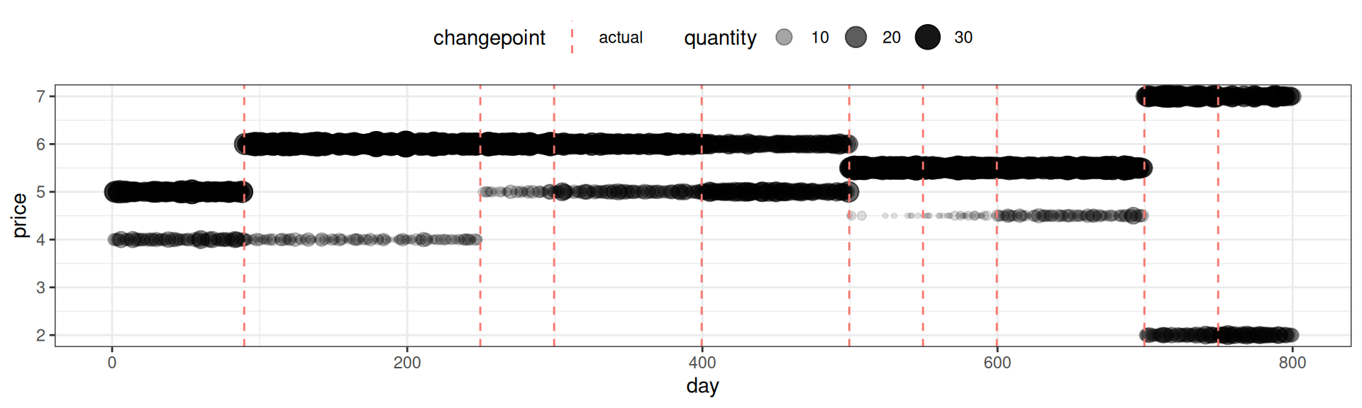
We define a segmentation of a histogram-valued time series \(h\) of length \(T\) as a vector \(z \in \{0, 1\}^{T-1}\), where \(z_t=1\) indicates a changepoint between indices \(t\) and \(t+1\), and \(0\) indicates its absence. From the index vector \(z\), we can derive a segmentation in the form of \(\mathcal{S}(z)\), i.e., a set of all segment intervals \([t_1, t_2]\).
The model is intended to select a segmentation \(z\) that best balances (i) goodness-of-fit (how well the empirical histograms are explained within segments) with (ii) model simplicity (how many changepoints are included). The balance is governed by the regularizing parameter \(\lambda\), which is selected by optimizing the posterior likelihood over it.
The posterior over a changepoint configurations \(z\) is assumed to be:
\[ p(z \mid \mathbf{n}, \lambda) \propto p(\mathbf{n} \mid z) \cdot p(z) \cdot p(\lambda) \]
The data likelihood is computed as the product of likelihoods of the segments defined by the segmentation \(\mathcal{S}(z)\), where \(\mathbf{n}_{[t_1, t_2]}\) stands for the histogram over the interval \([t_1, t_2]\).
\[ p(\mathbf{n} \mid z) = \prod_{(t_1, t_2) \in \mathcal{S}(z)} p(\mathbf{n}_{[t_1, t_2]})\text{,} \]
The likelihood of a segment \(\mathbf{n}_{[t_1, t_2]}\) is set to it (regularized) maximum likelihood estimate … (explain more) …, where \(\hat{p}_i\) is the (regularized) maximum likelihood estimate of the relative frequencies of the different price points. This corresponds to using the maximum likelihood estimate of the multinomial probabilities within each segment. Although technically this is not fully Bayesian (since we’re not integrating over latent parameters), it can be viewed as an empirical Bayes approximation.
\[ p(\mathbf{n}_{[t_1, t_2]}) = \sum_{i=1}^{K} (\hat{p}_i)^{n_i} \]
In computing \(\hat{p}_i\), we smooth each bin count with a small constant \(\epsilon\) to prevent division by zero.
\[ \hat{p}_i = \frac{n_i + \epsilon}{\sum_j (n_j + \epsilon)} \]
We place a Bernoulli prior on each potential changepoint, to penalize excessive complexity: small \(\lambda\) values encourage fewer changepoints, favoring parsimony. In consequence, the model selects the segmentation \(z\) that best balances goodness-of-fit (how well the empirical histograms are explained within segments) with model simplicity (how many changepoints are included). The balance is governed by \(\lambda\).
\[ z_t \sim \text{Bernoulli}(\lambda) \]
To estimate the changepoint configuration \(z\), we use a greedy forward search:
This process is repeated for different values of \(\lambda\), and the \(\lambda\) value that maximizes the resulting posterior is selected using one-dimensional optimization (optimize() in R).
This project implements a greedy changepoint detection algorithm for time series of price histograms. The codebase consists of three components:
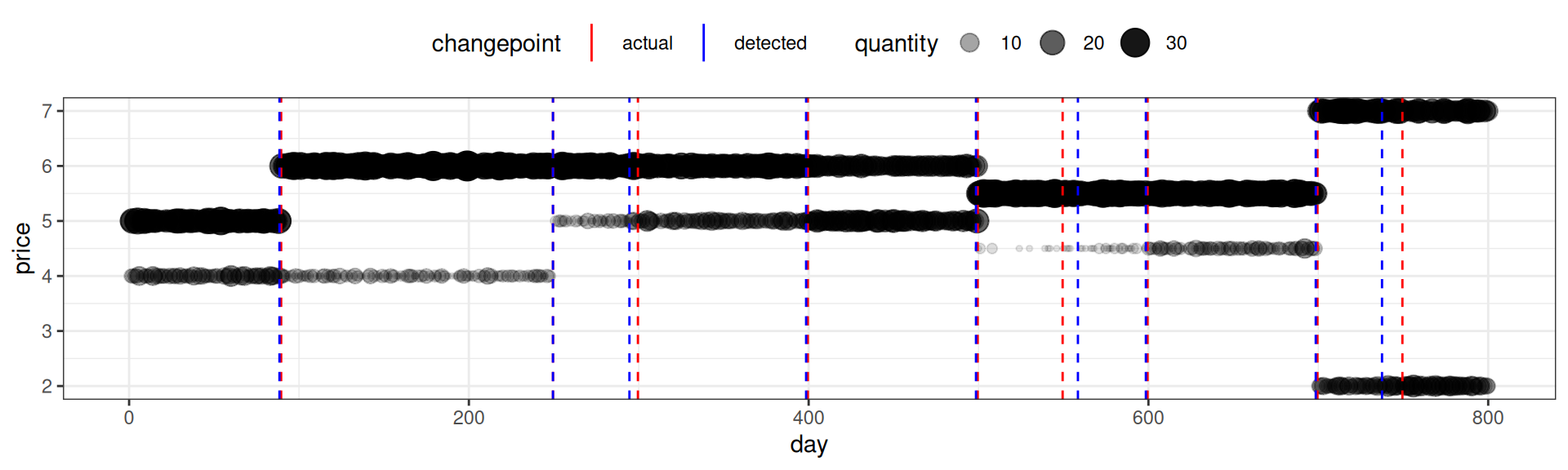
generate_transaction_prices()).compute_price_histogram()).In the present example, the algorithm detects the same number changepoints, and the estimates ones, are largely fairly close to the simulated ones. A formal evaluation is pending. It stands to reason that the accuracy of changepoint identification will depend on the similarity between adjacent segments, as well as segment length.
opt_res <- locate_optimal_changepoints( hist$histogram, max_lambda = 0.3 )
detected_changepoints <- which(opt_res$changepoints) - 0.5

knitr::kable(t(actual_changepoints), caption = "Original Changepoints")| 89.5 | 249.5 | 299.5 | 399.5 | 499.5 | 549.5 | 599.5 | 699.5 | 749.5 |
knitr::kable(t(detected_changepoints), caption = "Detected Changepoints")| 88.5 | 249.5 | 294.5 | 398.5 | 498.5 | 558.5 | 598.5 | 698.5 | 737.5 |
The plot below illustrates the results vis a vis the simulation assumptions.
p_price +
      geom_vline( data = data.frame(x = detected_changepoints, changepoint = "detected"),
                  aes(xintercept = x, color = changepoint), linetype = "dashed") +
      scale_color_manual(name = "changepoint", values = c("detected" = "blue", "actual" = "red"),
                        guide = guide_legend(override.aes = list( linetype = "solid", size = 1))
                        )
All source code is available here:
👉 https://github.com/plogacev/case_studies/tree/main/pricedist_changepoints
double log1m_exp(double x)
{
if (x >= 0.0) stop("log1m_exp is undefined for x >= 0");
...
}